Import Templates

Import Templates

FAQs  | Feedback

 Step

  Action

  1

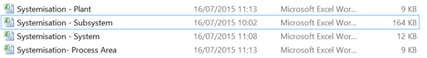
Creating separate datasheets for each level of systemization.

Creating separate datasheets for each level of systemization is mostly related to the systemization modules: Work Breakdown, Location Breakdown and Process Breakdown. Each level will need to be imported separately from the highest level to the lowest. E.g. when setting up the process breakdown, import a datasheet containing all Plants followed by Process Area, System and Subsystem. This is done because each level of systemization would need to be assigned to a parent systemization during each import, thus, the parent systemization would need to be set up first.

Splitting Datasheets.

 2

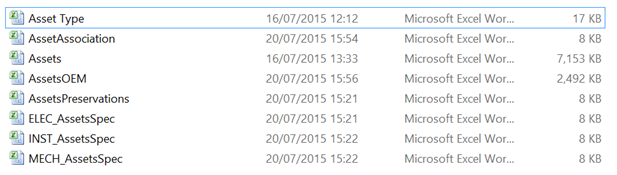
Splitting big datasheets into smaller chunks.

As mentioned before, breaking down import data into smaller pieces would allow for higher accuracy and efficiency but it would also increase the number of files and number of imports needed. A balance between speed and accuracy would need to be decided by the system administrator when creating these templates. In the example below, such a format would allow users to assign each import template to the relevant personnel as well as require the user to import a 1MB file into the system as opposed to a 50MB file.

Allow System to Assign IDs.

 3

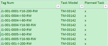
Allowing the system to assign IDs.

For certain modules, it is possible and recommended to allow the system to assign IDs to items. The problem with importing certain modules with a tag ID is that the tag ID may already exist for past items or other concurrent projects. This would not be an issue with certain modules such as Assets, Documents and Task Models which should have unique IDs within the company. For example, with multiple projects running at the same time within the system, it would be impossible for the multiple project teams to come up with unique Task IDs following the same protocol.

To instruct the system to assign an ID to an item, fill the column with one (1) alphabetical character. In the example below, the Planned Task would be assigned the next possible unique ID by the system thus ensuring there will not be any repeated IDs.

Excel Commands.

 4

Useful Excel Commands.

• =CONCATENATE (text1, [text2], …)

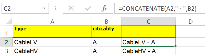
The concatenate function within excel is used to combine two (2) or more fields into one (1). This is useful when trying to create a column for “Summary” fields which are a combination of both the ID and Description or for other modules that require concatenation to simplify data manipulation.

Note: The use of spaces is very important when importing data from an excel sheet especially within Key Fields where an extra space or lack of one could result in data not being mapped to the correct item.

• =VLOOKUP (lookup_value, table_array, col_index_num, [range_lookup])

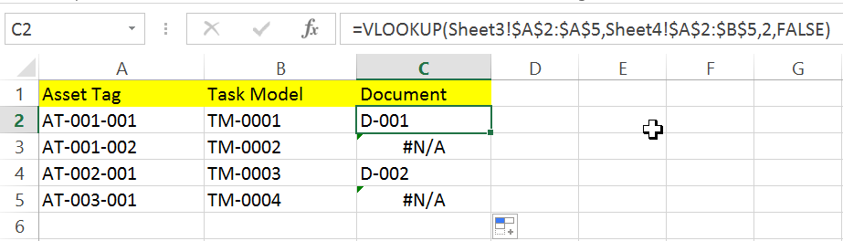
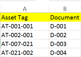
The vlookup function is used to find things in a table or range by row. For example, an Asset ID is assigned to both Task Models and Documents. Using the vlookup function will allow users to find all documents related to the task models through the assets (Good templates should not require you to refer to other documents for information you want but we will use this an example).

The vlookup function uses the Asset Tag as a reference point to pull data from the document data sheet into the task model data sheet so that the relationship between the Task Models and Documents are known.

Lookup_value:  The value you want to look up. The value must be in both datasheets so that it can be used as a reference point. The lookup_value should be the first column in the table_array.

Table_array:  The range of cells in which VLOOKUP will search for the lookup_value and the return value.

Col_index_num:  The column number (starting from 1 for the left-most column of table_array) that contains the return value.

Range_lookup:  True assumes the first column is sorted either numerically or alphabetically, and will search for the closest value. This is the default method if you don’t specify one.  False searches for the exact value in the first column.

Index and Match (Similar to vlookup but for more than 1 column)

The INDEX function returns the value of a specified cell selected by the row and column number index while the MATCH function searches for a specified item in a range of cells and returns the relative position of that item in the range. Together, these functions allow us to conduct a command similar to that of vlookup but with 2 or more criteria columns.

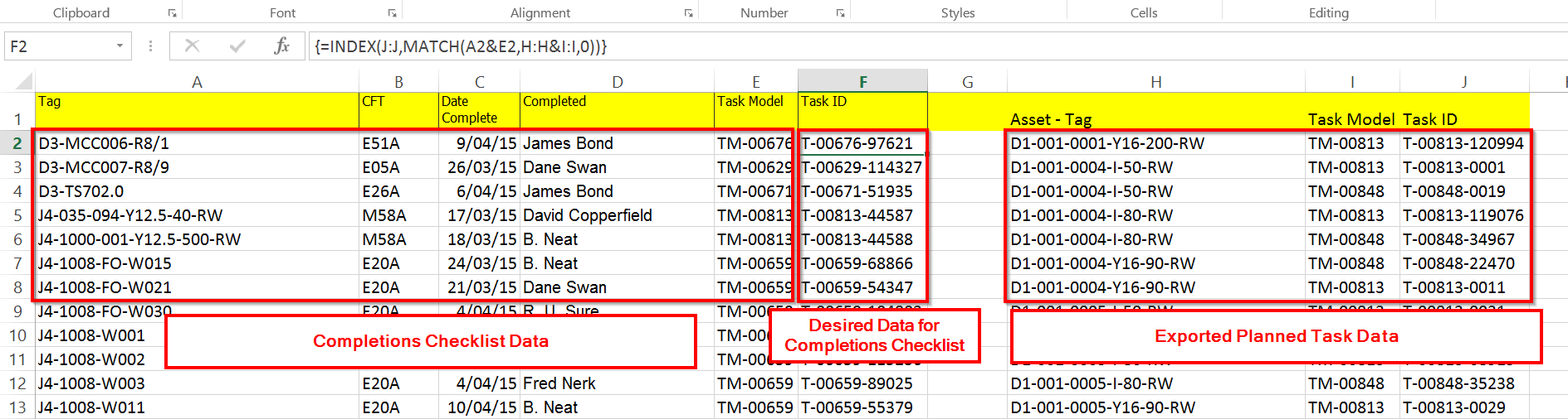
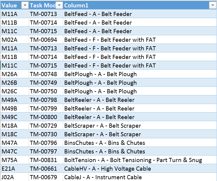
In this example, I needed to put in the Task ID into my list of completed checks that came with Asset Tag and Task Model. I exported my Planned Task data consisting of Asset – Tag, Task Model and Task ID as can be seen in the 3 columns on the right. The Index and Match functions allow me to cross reference the Asset Tag and Task Model from the completed check list with the Asset – Tag and Task Model from the Planned Task data to pump in Task IDs into the completed check list.

• =INDEX(array, row_num, [column_num])

Array:  The range of cells that contains the return value

Row_ num:  Selects the row in array from which to return a value.

Column_num:  Selects the column in array from which to return a value. Optional.

In this situation, we would use the MATCH function to provide the row_num for the INDEX function.

• =MATCH(lookup_value, lookup_array, [match_type])

Lookup_value:  The value that you want to match in lookup_array

Lookup_array:  The range of cells to be searched

Match_type:  The number -1, 0 or 1 which specifies how Excel matches the Lookup_value and Lookup_array. Optional.

In the example above, follow the steps listed below:

1. Sort the Exported Planned Task Data so that the Asset Tags are in order. There could be repeats in Asset Tags because there could be multiple Planned Tasks assigned to an Asset Tag.

2. Under Task ID, type in the following code in F2 and enter the code using CTRL+SHIFT+ENTER

=INDEX(J:J, MATCH(A2&E2, H:H&I:I, 0))

       J:J returns Task IDs from the Exported Planned Task Data

       A2&E2 concatenates the Asset Tag and Task Model from the Completed Checklist Data

       H:H&I:I concatenates the Asset Tag and Task Model from the Exported Planned Task Data

       The MATCH function matches the concatenated data from A2&E2 and H:H&I:I to provide the row number where the data matches

       The INDEX function will pump out the Task ID from array J:J from the row number provided by the MATCH function.

3. Drag down the INDEX and MATCH function to populate the rest of the Task ID column.

• Reverse Pivot Table

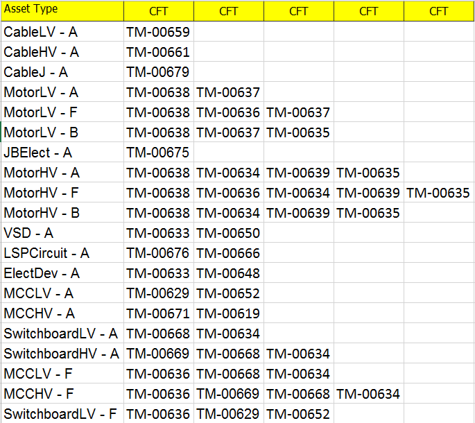
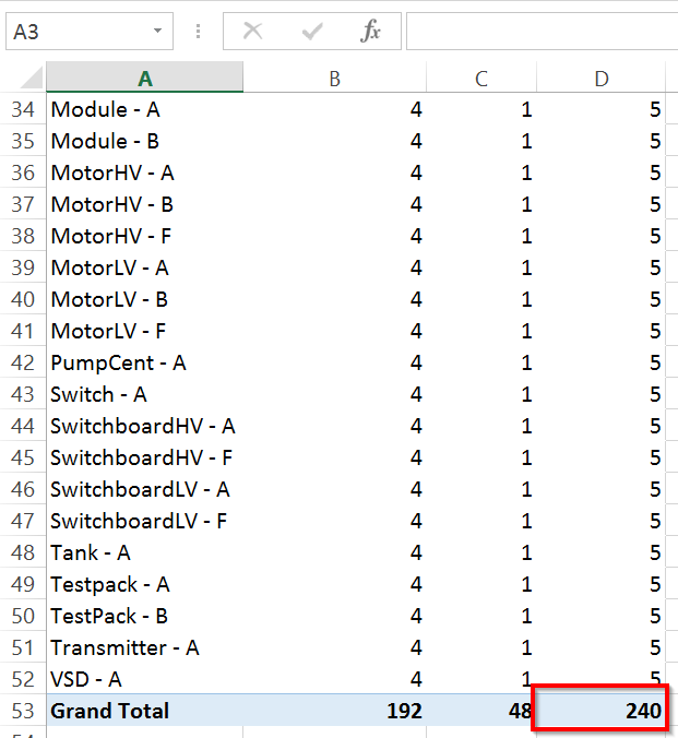
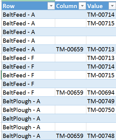
The Reverse Pivot Table function is useful for converting data from a matrix table to a data table which can be imported into the CE system. In the example above, Task Models were assigned to Asset Types in a matrix form. To import this data into the system, we had to list down each Asset Type with its allocated Task Model. To do this, follow the steps below:

1. Call for the PivotTable and PivotChart Wizard using ALT+D+P
2. Select “multiple consolidation ranges” for the data you want to analyse in Step 1 of 3.
3. Select “I will create the page fields” in Step 2a of 3.
4. Highlight the entire matrix table (without column header) and add it into the worksheet range in Step 2b of 3. Select 0 page fields.
5. Select where you want the generated PivotTable to appear, either is fine.
6. Double-click the Grand Total row of the Grand Total Column.

7. A new sheet will appear with a new table with the desired data list. The table would need a bit of cleaning up such as removing the “Column” column and removing the extra rows with no values.

Next Training:  Import Asset List

CONFIDENTIAL - Licensed Users Only